A plot() produces a single visualisation and consists of one or more marks—graphical primitives such as bars, areas, and lines—which serve as chart layers. Each plot has a dedicated set of encoding channels with named scale mappings such as x, y, color, opacity, etc.
Below we’ll describe the core semantics of plots and the various ways you can customize them.
Basics
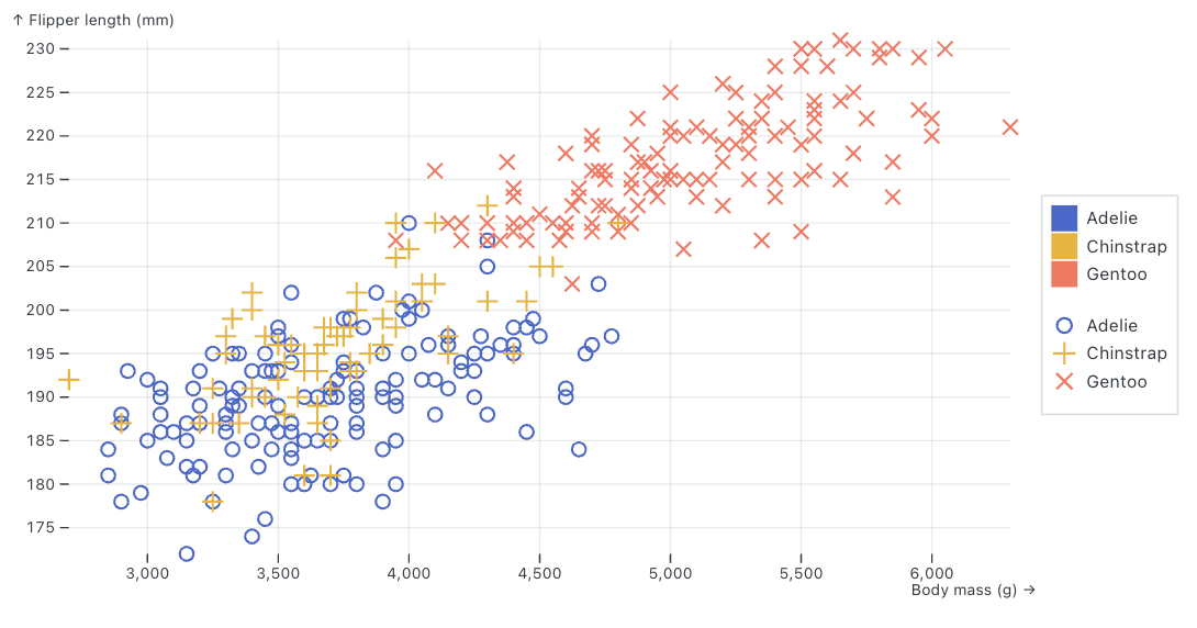
Here is a simple dot plot that demonstrates some key concepts (click on the numbers at right for additional details):
dot() mark for a simple dot plot, using a distinct stroke and symbol to denote the “species” column.
2
Legend in the default location, keyed by symbol.
3
Additional attributes that affect plot size and appearance.
Facets
Plots support faceting of the x and y dimensions, producing associated fx and fy scales. For example, here we compare model performance on several tasks. The task_name is the fx scale, resulting in a separate grouping of bars for each task:
Define legend using legend() function (to enable setting location and other options).
3
Remove default x labeling as it is handled by the legend.
4
Tweak y-axis with shorter label and ensure that it goes all the way up to 1.0.
Marks
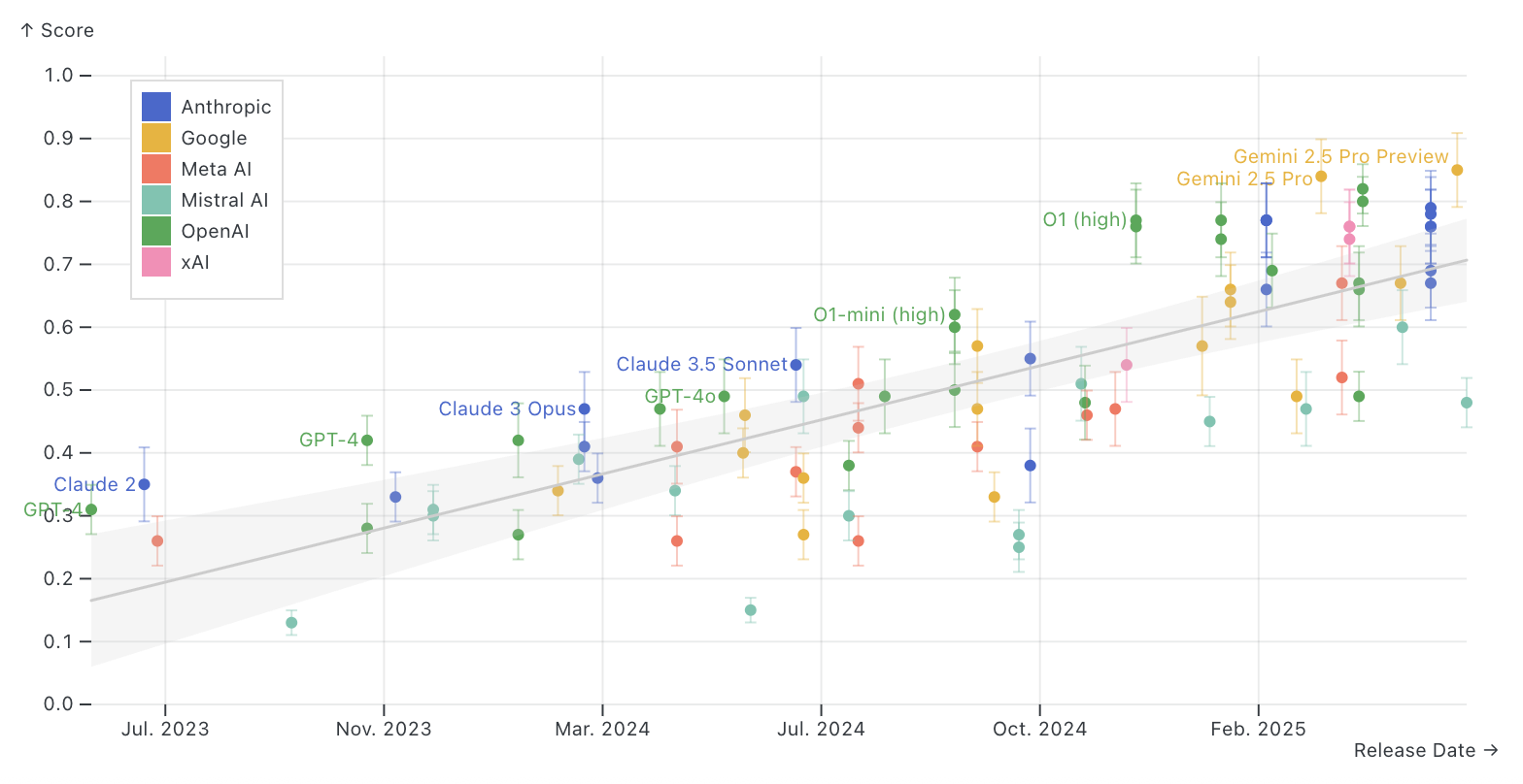
The plots above use only a single mark (dot() and bar_y() respectively). More sophisticated plots are often constructed with multiple marks. For example, here is a plot that adds a regression line mark do a standard dot plot:
Use fill to distinguish male and female athletes; use opacity to deal with a large density of data points.
2
Use stroke to ensure that male and female athletes each get their own regression line.
Tooltips
Tooltips enable you to provide additional details when the user hovers their mouse over various regions of the plot. Tooltips are enabled automatically for dot marks (dot(), dot_x(), dot_y(), circle(), and hexagon()) and cell marks (cell(), cell_x(), etc.) and can be enabled with tip=True for other marks. For example:
Add tip=True to enable tooltips for marks where they are not automatically enabled.
Note that tooltips can interfere with plot interactions—for example, if your bar plot was clickable to drive selections in other plots you would not want to specify tip=True.
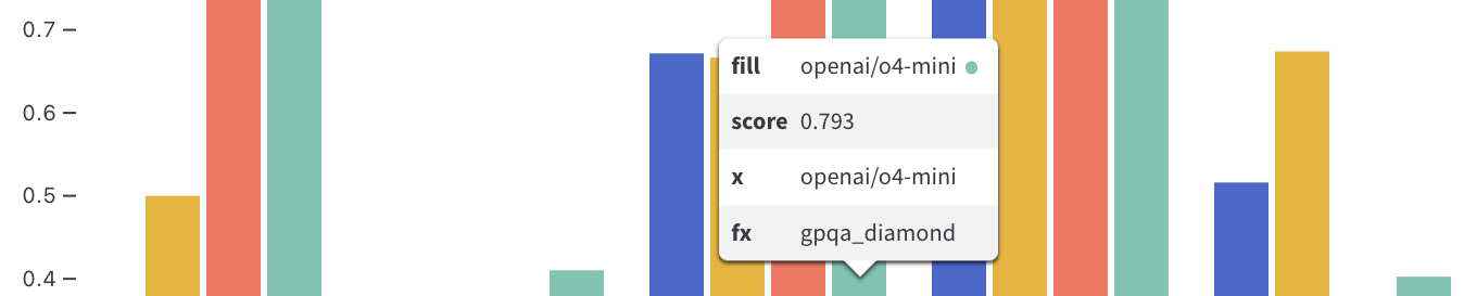
Channels
As illustrated above, tooltips show all dataset channels that provide scales (e.g. x, y, fx, stroke, fill, symbol, etc.). There are a few things we do to improve on the default display:
The labels are scale names rather than domain specific names (e.g. “fx” rather than “model”)
The order of labels isn’t ideal.
There are some duplicate values (e.g “fill” and “fx”)
We might want to include additional columns not used in the rest of the plot (e.g. a link to the log file).
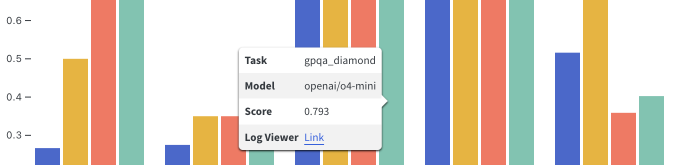
You can exercise more control over the tooltip by specifying channels along with the mark. For example:
The channels option maps labels to columns in the underlying data—all defined channels will appear in the tooltip. URL values are automatically turned into links as shown here.
Titles
Plot titles can be added using the title option. For example, here we add a title at the top of the frame:
If you have facet labels on the top of the x-axis, you may need to provide some additional top_margin for the title so that it is placed above the facet labels. Use the title() function to customize this:
from inspect_viz.mark import titleplot( ... title=title("Olympic Athletes", margin_top=40), ...)
You can also customize the font size, weight, and family using the title() function.
Axes
There are several options available for controlling the domain, range, ticks, and labels for axes.
Labels
By default axes labels are taken from the columns they are mapped to. Specify an x_label or y_label to override this:
If you want no axes label at all, pass None. For example:
plot( ..., x_label=None)
Domain
By default, the x and y axes have a domain that matches the underlying data. For example, if the data ranges from 0 to 0.8 the axes will reflect this. Set a specific x_domain or y_domain to override this. For example, here we specify that we want the y-axis to span from 0 to 1.0:
plot( ..., y_domain=[0,1.0])
You can also specify “fixed” for a domain, which will preserve the domain of the initial values plotted. This is useful if you have created filters for your data and you want the axes to remain stable across filtering. For example:
plot( ..., y_domain="fixed")
Ticks
You can explicitly control the axes ticks using the x_ticks and y_ticks options. For example, here we specify ticks from 0 to 100 by 10:
plot( ..., x_ticks=range(0, 100, 10))
If you want no ticks at all specify [], for example:
plot( ..., x_ticks=[])
There are several other tick related options. Here
[x,y]_tick_size — The length of axis tick marks in pixels.
[x,y]_tick_rotate — The rotation angle of axis tick labels in degrees clockwise.
[x,y]_tick_spacing — The desired approximate spacing between adjacent axis ticks, affecting the default ticks.
[x,y]_tick_padding — The distance between an axis tick mark and its associated text label.
[x,y]_tick_format — How to format inputs for axis tick labels (a d3-format or d3-time-format).
Sorting
You may sort a mark’s index, which changes the effective order of the data presented by that mark. This is useful for two scenarios:
Sorting an ordinal scale (for example, sorting the x or y axis to control the order in which elements are arranged). For example, in the heatmap implementation, we sort the x and y axis in order to position the highest score values in the top right corner of the heat map:
This example will sort the ordinal values of each axes.
Sorting the entire dataset to control the order in which the marks are drawn. This effectively controls the z-index of the mark, making it useful when there are overlapping marks and you’d like to control the order.
Legends are by default placed in a bordered box. Use the border and background options to control box colors (specifying False to omit border or background color). For example:
You may can pass multiple legends (strings like “color” or calls to legend()) to the plot() funciton. Each may be positioned independently using frame_anchor and inset, or if they share a position, the legends will be merged into a container in that location.
For example, the following adds two legends in the same container in the default position ( right of the plot):
Legends also act as interactors, taking a bound Selection as a target parameter. For example, discrete legends use the logic of the toggle interactor to enable point selections. Two-way binding is supported for Selections using single resolution, enabling legends and other interactors to share state.
See the docs on Toggle interactors for an example of an interactive legend.
Legend Name
The name directive gives a plot a unique name. A standalone legend can reference a named plot legend(..., for_plot="penguins") to avoid respecifying scale domains and ranges.
Baselines
Baselines can be including baseline() marks in the plot definition (or by including them in the marks option of pre-built views).
For example, here we add a baseline with the median weight from the athletes data:
If you have a simple static baseline, you may simply provide the value, along with other options to customize the label, position, and other attributes of the baseline. You can also use a tranformation function like median() to define baselines:
By default, baselines are drawn using the x-axis values. To draw a baseline using the y-axis values, pass orientation="y" to the baseline function.
Margins
Since the text included in axes lables is dynamic, you will often need to adjust the plot margins to ensure that the text fits properly within the plot. Use the margin_top, margin_left, margin_right, and margin_bottom options to do this. Note that there are also facet_margin_top, facet_margin_left, etc. options available.
For example, here we set a margin_left of 100 pixels to ensure that potentially long model names have room to display:
plot( data, bar_y(...), margin_left=100)
Colors
Use the color_scheme option to the plot() function to pick a theme (see the ColorScheme reference for available schemes). Use the color_range option to specify an explicit set of colors. For example, here we use the “tableau10” color_scheme:
In the examples above we made Data available by reading from a parquet file. We can also read data from any Python Data Frame (e.g. Pandas, Polars, PyArrow, etc.). For example:
import pandas as pdfrom inspect_viz import Data# read directly from filepenguins = Data.from_file("penguins.parquet")# read from Pandas DF (i.e. to preprocess first)df = pd.read_parquet("penguins.parquet")penguins = Data.from_dataframe(df)
You might wonder why is there a special Data class in Inspect Viz rather than using data frames directly? This is because Inpsect Viz is an interactive system where data can be dynamically filtered and transformed as part of plotting—the Data therefore needs to be sent to the web browser rather than remaining only in the Python session. This has a couple of important implications:
Data transformations should be done using standard Python Data Frame operations prior to reading into Data for Inspect Viz.
Since Data is embedded in the web page, you will want to filter it down to only the columns required for plotting (as you don’t want the additional columns making the web page larger than is necessary).
Selections
One other important thing to understand is that Data has a built in selection which is used in filtering operations on the client. This means that if you want your inputs and plots to stay synchoronized, you should pass the same Data instance to all of them (i.e. import into Data once and then share that reference). For example:
from inspect_viz import Datafrom inspect_viz.plot import plotfrom inspect_viz.mark import dotfrom inspect_viz.inputimport selectfrom inspect_viz.layout import vconcat# we import penguins once and then pass it to select() and dot()penguins = Data.from_file("penguins.parquet")vconcat( select(penguins, label="Species", column="species"), plot( dot(penguins, x="body_mass", y="flipper_length", stroke="species", symbol="species"), legend="symbol", color_domain="fixed" ))
SQL
You can use the sql() transform function to dynamically compute the values of channels within plots. For example, here we dynamically add a bias parameter to a column:
Any valid SQL expression can be used. For example, here we use an IF expression to set the stroke color based on a column value:
stroke=sql(f"IF(task_arg_hint, 'blue', 'red')")
Dates
Numeric Values
In some cases your plots will want to deal with date columns as numeric values (e.g. for plotting a regression line). For this case, use the epochs_ms() transform function to take a date and turn it into a timestampm (milliseconds since the epoch). For example:
In some cases you may have timeseries data which you’d like to reduce across months or years (e.g.collapse year values to enable comparison over months only). The following transformations can be used to do this:
Transform a Date value to a month boundary for cyclic comparison. Year values are collapsed to enable comparison over months only.
date_day_month()
Map date/times to a month and day value, all within the same year for comparison.
Attributes
Attributes are plot-level settings such as width, height, margins, and scale options (e.g., x_domain, color_range, y_tick_format). Attributes may be Param-valued, in which case a plot updates upon param changes.
Some of the more useful plot attribues include:
width, height, and aspect_ratio for controlling plot size.
margin and facet_margin (and more specific margins like margin_top) for controlling layout margins.
style for providing CSS styles.
aria_label and aria_description, x_aria_label, x_aria_description, etc. for accessibilty attributes.
x_domain, x_range,y_domain, andy_range` for controlling the domain and range of axes.
Tick settings for x, y, fx, and fy axes (e.g. x_ticks, x_tick_rotate, etc.)
r (radius) scale settings (e.g. r_domain, r_range, r_label, etc.)
See PlotAttributes for documentation on all available plot attributes.